Sketchnote
One-page summary
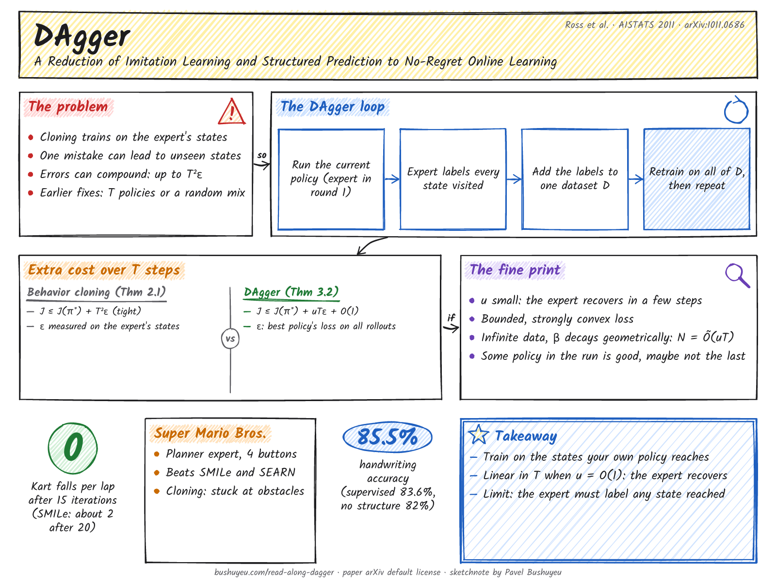
A Reduction of Imitation Learning and Structured Prediction to No-Regret Online Learning. Ross, Gordon and Bagnell, AISTATS 2011.
Summary
DAgger (Dataset Aggregation) learns from an expert in rounds: run the current policy, let the expert label the states it visits, add them to one growing dataset, and retrain on all of it.
Analysed as no-regret online learning, this finds a stationary, deterministic policy whose extra cost over the expert is at most uTε_N + O(1) (Theorem 3.2), where ε_N is the best single policy's loss on the states the training runs visited. This is linear in the horizon T when u, the extra cost of one mistake, is O(1); behavior cloning's bound is T²ε, with ε measured on the expert's states.
In Super Tux Kart, Super Mario Bros. and handwriting recognition it beats behavior cloning and SMILe, with a Kart policy that never falls off the track after 15 iterations and 85.5% character accuracy against 83.6%.
One-page summary
In class
Keep these in mind while the presenter talks. Tick them on page 2 of the PDF as they come up.
FAQ
No, it is tight. Theorem 2.1 bounds the extra cost of a policy trained only on the expert's states by T²ε, and the paper cites problems where the extra cost really grows as T²ε, such as Ross and Bagnell's example with J(π̂_sup) = (1 − εT)J(π*) + T²ε. The cause is compounding: after a mistake, the learner may reach states that the expert's data does not cover, and its errors add up. (Sec. 1, Sec. 2.1, Theorem 2.1)
No. For a general task cost C in [0, 1], with ℓ an upper bound on the 0-1 loss and the other assumptions of Theorem 3.2, some learned policy satisfies J(π̂) ≤ J(π*) + uTε_N + O(1), where u bounds how much one wrong action, followed by the expert, can add to the cost-to-go. u ≤ 1 when the cost is disagreement with the expert, and u = O(1) when the expert gets back on track within a few steps. In the worst case u is O(T), and the bound is no better than behavior cloning's. (Sec. 2.2, Theorems 2.2 and 3.2)
No. In T²ε (Theorem 2.1), ε is the policy's loss on the expert's state distribution. In DAgger's bounds, ε_N is the loss of the best single policy in hindsight on the states that the training policies visited, which include states the expert never reaches. The paper links the two with an assumption: for any input distribution, some policy in the class reaches loss ε. (Sec. 2.1, Sec. 3, Sec. 4.2)
Only in the first round of the simplest version. With β_i = I(i = 1), the expert's actions run the system in iteration 1 only; after that the learned policy acts, and the expert labels each visited state with the action it would take. So the expert must be able to label states it would never reach itself: in the paper, a human who gives the correct steering for Super Tux Kart images, and a planner with full game state in Mario. (Sec. 3, Algorithm 3.1, Sec. 5.1–5.2)
β_i is the probability that the expert, not the learner, picks the control while data is collected in iteration i, and it is optional. For convergence in the limit, the theory needs only the average of the β_i to go to 0; the iteration counts of Theorems 3.1–3.4 assume the stronger β_i ≤ (1 − α)^(i−1). The analysis pays for β through the gap between the state distributions of the mixed and the learned policy (at most 2Tβ_i, Lemma 4.1). In practice the parameter-free β_i = I(i = 1) often works best; in Mario, β_i = 0.5^(i−1) did slightly better (3030 against 2980 distance per stage) and 0.9^(i−1) converged much more slowly. (Sec. 3, Lemma 4.1, Theorem 4.1, Sec. 5.2)
Not necessarily the last one. Each theorem says that some learned policy among π̂_1 ... π̂_N does well under its own state distribution, for example the best of them. Footnote 3 adds that the same guarantee holds, on average, for a policy that picks one of them uniformly at random and runs it for T steps; a single draw can still be a bad policy. Algorithm 3.1 returns the best policy on validation data. (Theorem 3.1, footnote 3, Algorithm 3.1)
In theory, with a bounded, strongly convex loss and β_i ≤ (1 − α)^(i−1) for a constant α independent of T, infinite data per iteration needs N = Õ(T) for the surrogate-loss bound (Theorem 3.1) and Õ(uT) for the task-cost bound (Theorem 3.2). With a constant number of sampled trajectories per iteration, the two bounds need N = O(T² log(1/δ)) and O(u²T² log(1/δ)), with probability at least 1 − δ (Theorems 3.3–3.4); the paper says a sharper analysis may bring the first down to Õ(T log(1/δ)), but does not prove it. The experiments all run 20 iterations, and in Super Tux Kart DAgger almost never falls after 5 and never falls after 15. (Sec. 3, Theorems 3.1–3.4, Sec. 5)
An online learner is no-regret if its average loss over the iterations approaches that of the best fixed policy in hindsight (Eq. 3). Retraining on the aggregated data is Follow-The-Leader, which is no-regret for strongly convex losses, and the analysis uses only that property. So imitation learning reduces to no-regret online learning: give any no-regret algorithm the loss on the states visited by each iteration's policy, and Theorem 4.1 bounds the loss by ε_N plus its average regret γ_N and a penalty for β, so the iterations needed depend on how fast γ_N falls. The paper notes this needs more than the classification-only reductions behind SEARN and SMILe: a no-regret method or a strongly convex loss. (Sec. 3, Sec. 4.1–4.2)
DAgger trains each new policy on all the data collected so far, then returns one stationary, deterministic policy picked on validation data. Forward training learns a separate policy for each of the T time steps over T iterations, which is impractical when T is large or undefined; SMILe and SEARN return a stochastic mixture that adds one policy per iteration, and the cited SMILe result gets near-linear regret on some problem classes with α in O(1/T²) and N in O(T² log T) iterations. In Super Tux Kart, SMILe still fell off about twice per lap after 20 iterations, partly because its stochastic policy sometimes picks bad actions; in Mario, DAgger beat SEARN for every α tried. (Sec. 1, Sec. 2.2–2.3, Sec. 5.1–5.2)
No. The supervised baseline also gets more data, all from the expert's own trajectories, and its performance does not improve in Super Tux Kart and stagnates in Mario. The paper's reason: the expert's laps are alike and never show how to recover, and in Mario the expert jumps early, so the cloned policy never learns to get unstuck next to an obstacle. DAgger and the other iterative methods add data from the states their own policies reach, including those stuck positions. (Sec. 5.1–5.2, Figs. 2 and 4)
Following SEARN (Daumé III et al.), the paper treats structured prediction as imitation learning with trivial dynamics: letters are predicted left to right, and the previous predicted letter is an input to the next prediction. Training with the true previous letter is the supervised approach (83.6% character accuracy, against 82% with no structure); DAgger trains on its own previous predictions and reaches 85.5%. SEARN with α = 0.8 or α = 1 does about as well as DAgger here; the paper notes that only the previous-letter feature depends on the policy, so pure policy iteration stays stable on this task. (Sec. 5.3, Fig. 5)
They do not test a physical robot or a large model. All learners are linear (ridge regression in Kart, linear SVMs in Mario and handwriting) on simple features: downsampled pixels, hand-coded grid cells and binary pixels. Kart uses one track (Star Track) and Mario only difficulty-1 stages. Most comparisons are curves; the text gives only a few numbers: SMILe's about 2 falls per lap, 2980 and 3030 in Mario, and 82%, 83.6% and 85.5% in handwriting. (Sec. 5, Figs. 2, 4 and 5)
Glossary
Links
How this page was made. The video is an AI narration (Breeze TTS 2) of the full paper with the text on screen. The summary, questions and sketchnote were drafted with an AI assistant from the paper's text and checked against it; the references in brackets point to the paper. Paper license: arXiv default license. The sketchnote is an original drawing, not a copy of the paper's figures.